LLM Systems Catch-Up Series - Transformer

Since the release of ChatGPT at the end of 2022, Large Language Models (LLMs) have captured widespread public attention. Thanks to their remarkable reasoning capabilities, LLMs have unlocked a plethora of downstream applications. Over the past two years, these models have evolved rapidly—from GPT-3.5 to DeepSeek R1—paving the way for advanced long thinking. Concurrently, serving systems like vLLM and SGLang have also seen rapid development, enabling efficient and scalable inference.

Inspired by this wave of innovation, I’ve decided to dive deeper into the world of LLMs by reading a series of research papers and documenting my insights and reflections. Assuming you have a foundational understanding of deep learning concepts, my goal is to build on that knowledge and explore the intricacies of LLMs in a way that’s both accessible and insightful. My hope is that this effort will serve as a helpful resource for others who are equally eager to explore this exciting field.

In this first blog, I’ll dive into the key component of LLMs: the Transformer¹, a groundbreaking architecture introduced by Google in 2017. The Transformer is a self-attention model that captures the contextual relationships between tokens.

Tokens and Autoregressive Generation

Tokens are the fundamental units of input and output in LLMs, created by splitting sentences into smaller segments, such as words or subwords. The Transformer operates in an autoregressive manner, meaning it generates tokens one at a time. At each step, it takes the current sequence as input, predicts the next token, and appends that token to the sequence to form the next input. For example, if the model is generating the sentence “The cat is on the mat,” the process might look like this:

• Input: [Start] → Output: “The”
• Input: “The” → Output: “cat”
• Input: “The cat” → Output: “is”
• Input: “The cat is” → Output: “on”
• Input: “The cat is on” → Output: “the”
• Input: “The cat is on the” → Output: “mat”

Here, [Start] is a special token used to indicate the beginning of the sequence, allowing the model to initiate the generation process. This step-by-step process continues until the model generates a complete sentence or reaches a stopping condition.

Next, let’s take a closer look at the architecture of the Transformer to gain a high-level understanding.

Architecture

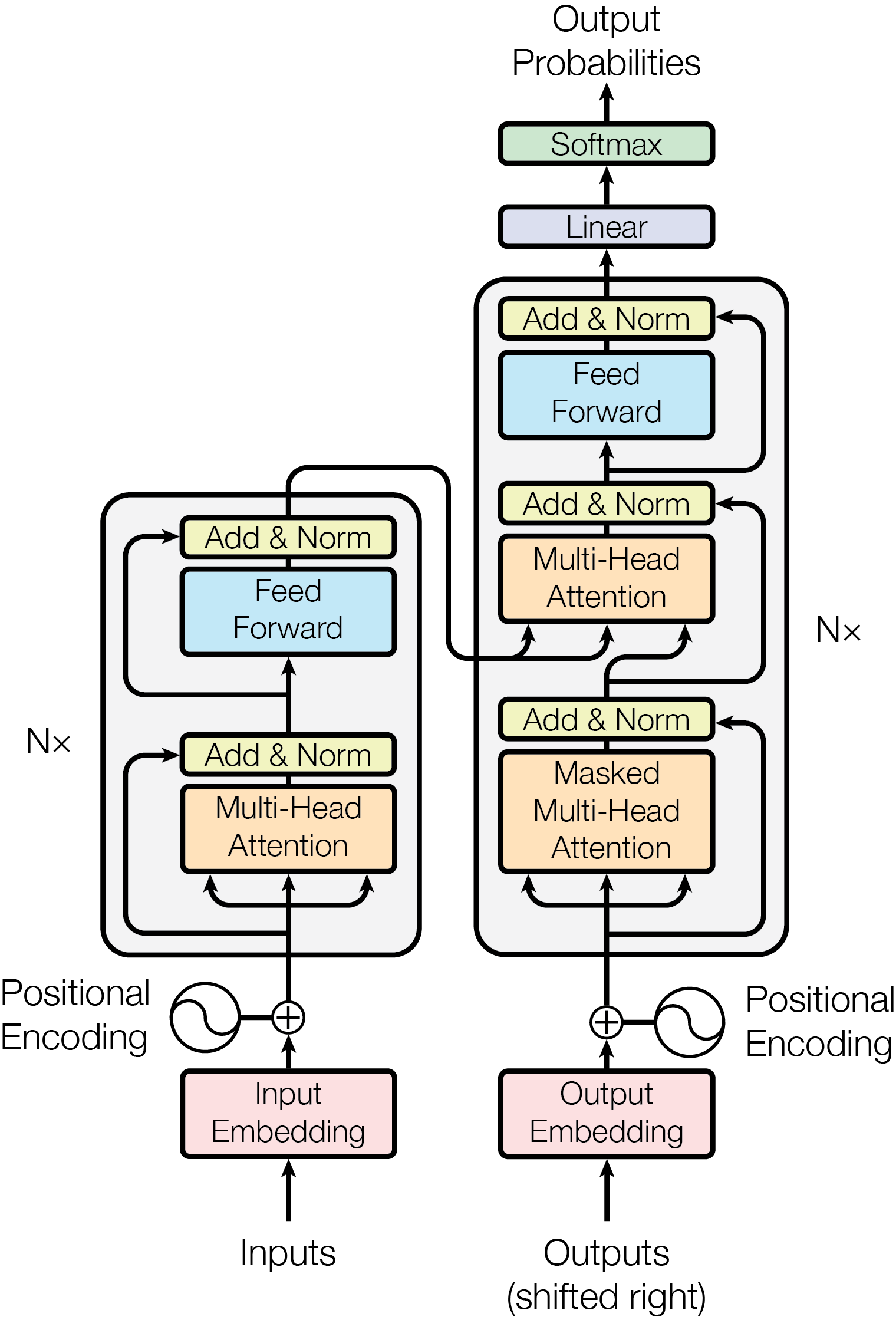
As shown in the figure above, the Transformer is composed of two main components: the Encoder and the Decoder. The Encoder maps the input sequence into a set of features, while the Decoder generates the output sequence token by token, using the features from the Encoder and the previously generated tokens. For example, in an English-to-German translation task, if the input sequence is “The cat is on the mat,” the Encoder processes this sequence into a set of feature representations. The Decoder then uses these features, along with the previously generated tokens (e.g., “Die Katze ist”), to predict the next token (e.g., “auf”) and ultimately produce the full output sequence: “Die Katze ist auf der Matte.”

Both the Encoder and Decoder consist of multiple stacked blocks. Each block contains one or two Multi-Head Attention layers and a Feed Forward layer. These layers are wrapped by a residual connection, implemented as: $\text{LayerNorm}(x + \text{Sublayer}(x))$, where $\text{Sublayer}$ can be either the Multi-Head Attention or Feed Forward layer. $\text{LayerNorm}$ (Layer Normalization) normalizes the data to have a mean of $0$ and a variance of $1$, which stabilizes training and accelerates convergence by reducing internal covariate shift.

Looking at the architecture, a natural question arises:

📝 Why is an Encoder necessary? Can the task be achieved using only the Decoder?

The Transformer was originally designed for machine translation tasks, where the input (e.g., an English sentence) and output (e.g., a German sentence) are different sequences. In such cases, the Encoder-Decoder architecture is crucial because it allows the model to separately process the input and generate the output, ensuring better performance and accuracy. However, many recent models, such as GPT, use only the Decoder. This is because Decoder-only architectures are simpler, more scalable, and highly effective for tasks where the input and output sequences are the same, such as text generation.

Next, let’s take a closer look at each component shown in the architecture: Multi-Head Attention, Feed Forward, LayerNorm, Embedding, and Positional Encoding.

Attention

Multi-Head Attention

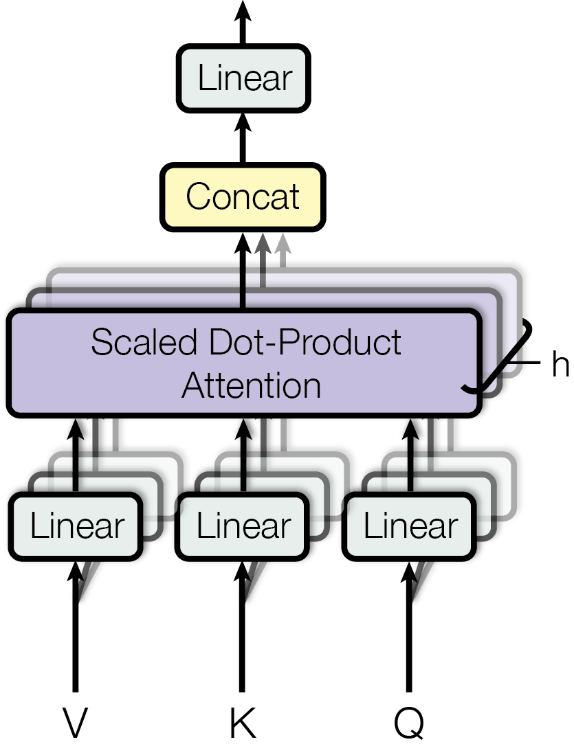
As illustrated in the above figure, the Multi-Head Attention has three inputs $V$ (values), $K$ (keys), and $Q$ (queries). These inputs are passed through a linear transformation and then fed into the Scaled Dot-Product Attention. Notably, there are $h$ copies of the linear and attention layers, which is where the term “multi-head” comes from. This design increases the network’s capacity and diversity, as each attention head can focus on learning different features. The resulting tensors from each attention head are concatenated and passed through a final linear layer.

Formally, Multi-Head Attention is defined as:

Here, $Q$, $K$, and $V$ have the size $n \times d_\text{model}$, where $n$ is the number of tokens (sequence length), and $d_\text{model}$ is the dimensionality of the model’s hidden states. The weight matrices $W_i^Q$ and $W_i^K$ have the size $d_\text{model} \times d_k$, and $W_i^V$ has the size $d_\text{model} \times d_v$, where $d_k$ and $d_v$ are the dimensionality of the keys/values and queries, respectively. In the original paper, $d_\text{model}$ is set to $512$, $d_k$ and $d_v$ are set to $64$, and the number of attention heads $h$ is set to $8$.

Scaled Dot-Product Attention

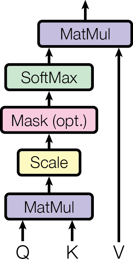
Within Multi-Head Attention, the Scaled Dot-Product Attention is the core component that computes the contextual relationships between tokens. It achieves this by performing a matrix multiplication between $Q$ and $K$, followed by a softmax layer to derive the attention scores between tokens. A higher attention score means that the model assigns the greater importance to the relationship between those tokens. These scores are then applied to $V$ to obtain a weighted sum of embeddings for each token.

Intuitively, the matrix multiplication between $Q$ and $K$ calculates the dot product between the embeddings of two tokens. The stronger relationship between the tokens, the higher the value of the dot product. Tokens with stronger relationships should naturally receive more attention, which is reflected in how the attention score are applied to $V$.

Formally, the Scaled Dot-Product Attention is defined as:

Here, $Q$, $K$, and $V$ have the sizes $n \times d_k$, $n \times d_k$, and $n \times d_v$, respectively. The symbol $\odot$ represents element-wise multiplication. $M$ is the causal mask, which prevents future tokens from influencing the computation of attention scores. This is essential in the Decoder, as autoregressive models generate tokens based solely on previous tokens. $M$ is a square matrix of size $n \times n$, defined as:

The full matrix looks like this:

The $i$-th row of $M$ determines which tokens can attend to the computation of the $(i+1)$-th token. For example, consider the second row of $M$, where the first and second columns are set to $1$, and the rest are $-\infty$. This means that when generating the third token, only the first and second tokens are involved in the computation of attention scores. This mechanism prevents the model from “cheating” by looking at future tokens during training or generation. Note that the masked values are set to $-\infty$ rather than $0$ so that they become $0$ after the softmax layer.

You may have noticed that in the definition, $QK^T$ is divided by a constant $\sqrt{d_k}$. Why is this?

📝 Why divide by $\sqrt{d_k}$?

It is for normalization. Assume each element in $Q$ and $K$ is a random variable with mean $0$ and variance $1$. Then each element in $QK^T$ is the dot product of a row from Q and K, which has mean $0$ and variance $d_k$. After dividing by $\sqrt{d_k}$, the variance becomes $1$, preventing gradient vanishing. Without this scaling, a large variance would mean some values are extremely large while others are extremely small, leading to gradients of $1$ for the largest values and $0$ for the smaller values (similar to the behavior of the $\text{max}$ function).

Now, let’s analyze the time complexity of Multi-Head Attention. For each attention layer, the computation involves $\mathcal{O}(n^2 (d_k + d_v))$. The projection of $Q$, $K$, and $V$ involves $\mathcal{O}(n \cdot d_\text{model} \cdot (d_k + d_v))$, and the final linear layer involves $\mathcal{O}(n \cdot d_\text{ff} \cdot (h \cdot d_v + d_\text{model}))$, where $d_\text{ff}$ is the hidden layer size. Note that the paper assumes $d_k = d_v$ and $d_k \times h = d_\text{model}$. Therefore, the total complexity simplifies to $\mathcal{O}(n \cdot d_\text{model} \cdot (n + d_\text{ff} + d_\text{model}))$. As a result, the Feed Forward layer dominates the computation for short sequences, while the Scaled Dot-Product Attention layer becomes the bottleneck for long sequences.

Having explored Multi-Head Attention, the next question is:

📝 What’s the advantage of the attention layer over a linear layer?

The attention layer models interactions between different tokens, while a linear layer process each token independently. Intuitively, the attention layer performs token-level mixing, capturing relationships between tokens, whereas the linear layer performs channel-level mixing, transforming features within each token.

Feed Forward

The outputs from the Multi-Head Attention layer are then passed to Feed Forward layer. This layer consists of two linear layers with a ReLU activation in between. The input and output dimensions are set to $d_\text{model} = 512$, while the hidden layer size is set to $d_\text{ff} = 2048$.

LayerNorm

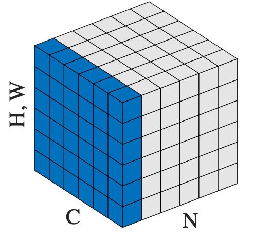
The outputs from both the Multi-Head Attention layer and the Feed Forward layer are then passed through a LayerNorm layer. LayerNorm functions similar to BatchNorm in that it normalizes the input data, but unlike BatchNorm, which normalizes across the batch dimension for each channel, LayerNorm normalizes across the feature dimension for each token. As shown in the figure, $N$ is the number of tokens, $C$ is the dimensionality of the embeddings, and $H/W$ is $1$. The blue part means that LayerNorm normalizes the embedding of each token individually. LayerNorm was chosen because it was essentially the standard at that time and empirically performed better than BatchNorm for machine translation tasks.

Now that we’ve explored everything in the transformer block, let’s dive deeper into the embedding and positional encoding.

Embedding

Embedding is the representation of the input sequence, as the original sequence cannot be processed directly by the neural network. It is obtained by tokenizing the sequence and passing it through an embedding layer.

The embedding layer acts as a lookup table, mapping each token to its corresponding embedding. The table has a size of $\text{vocab_size} \times \text{embedding_dim}$. The input is a list of token IDs, and the output is the corresponding embeddings of these tokens.

For example, let’s assume the input sequence “The cat is on the mat” is tokenized into $[464, 3797, 318, 319, 262, 2603]$, where each number corresponds to a token ID. These IDs are then passed to the embedding layer. The resulting matrix has $6$ rows, where each row is a copy of the corresponding row in the embedding weight matrix. Specifically, the first row is a copy of the $464$th row of the embedding weight, the second row is a copy of the $3797$th row, and so on.

In the Transformer, the embedding layer shares its weight with the pre-softmax linear layer. Although the weight size of the linear layer is $d_\text{model} \times \text{vocab_size}$, the weights can be shared by transposing them, since $\text{embedding_dim} = d_\text{model}$. It’s worth noting that the embedding weights are not directly borrowed from the linear layer but are obtained by multiplying the linear weight by $\sqrt{d_\text{model}}$. But why is this done?

📝 Why multiply the linear weights by $\sqrt{d_\text{model}}$

This scaling increases the embedding values before they are added to the positional encoding, making the positional encoding relative smaller. This ensures that the embedding vector isn’t overwritten by the positional encoding.

This weight-sharing design is truly clever, as it reduces the model size and eliminates the need for additional training of the embedding layers.

Positional Encoding

The embedding is then added to the positional encoding so that the tokens are aware of their positions in the sequence during the self-attention operation. Without positional information, the network cannot distinguish the order of the words and may misinterpret sentences. For example, consider the two sentences “The cat is on the mat” and “The mat is on the cat”. These sentences have the same words but opposite meanings due to the different word orderings.

The position encoding used in the Transformer is a combination of sine and cosine functions of different frequencies:

Here, $pos$ refers to the position of the token in the sequence, ranging from $0$ to $n-1$; $2i$ and $2i+1$ refer to the dimension in the embedding, ranging from $0$ to $d_\text{model}-1$.

To give a high-level understanding of the encoding function, I visualize the function:

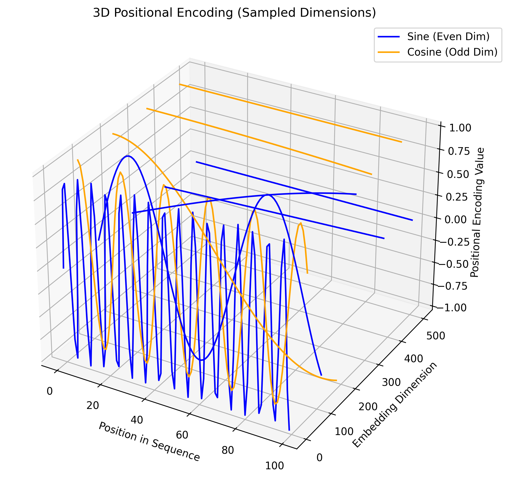
As shown in the figure, $8$ out of $512$ embedding dimensions are sampled and plotted, with even dimensions colored blue and odd dimensions colored orange. As the dimension increases, the wavelengths of the sine and cosine functions increase from $2\pi$ to $10000 \cdot 2\pi$.

This encoding function is designed to capture both absolute and relative positional information.

• Absolute Position: The wavelengths $10000^{\frac{2i}{d_\text{model}}} \cdot 2\pi$ are not integers, ensuring that two tokens at different positions never have the same positional encoding.
• Relative Position: The combination of sine and cosine implicitly encodes relative positional information. Specifically, the positional encoding of $pos + k$ can be represented as a linear transformation of the positional encoding of $pos$, based on trigonometric identities. For simplicity, assume the wavelengths are $2\pi$.

Therefore, both sine and cosine are necessary, as neither can achieve this independently. Additionally, the combination of different wavelengths is essential to capture dependencies over different ranges: short wavelengths capture short-range dependencies, while long wavelengths capture long-range dependencies. The base $10000$ is set empirically—it cannot be too small (redundant encoding, poor long-range dependency) or too large (poor short-range dependency).

The above explains the reasoning behind the encoding function. This leads to the following question:

📝 Why can’t simple encodings like $\{0, 1, \ldots, n-1\}$ or $\{0, 1/n, \ldots, (n-1)/n\}$ be used?

These encodings do not generalize to different sequence lengths, as they depend on the sequence length.

References: